Modelling Geographic Atrophy Progression using Implicit Neural Representations

Simone Sarrocco^1,2, Paul Friedrich¹, Florentin Bieder¹, Christina Bornberg⁴, Philippe Valmaggia^1,2,3 Peter M. Maloca^1,2,3,* Philippe C. Cattin^1,*

¹Department of Biomedical Engineering, University of Basel, Allschwil, Switzerland ²Department of Ophthalmology, University Hospital Basel, Basel, Switzerland ³Moorfields Eye Hospital NHS Foundation Trust, London, United Kingdom ⁴Vienna University of Natural Resources and Life Sciences, Vienna, Austria ^*Shared last authorship

ArXiv Code

Abstract

Age-related Macular Degeneration (AMD) is the major cause of blindness in the Western world. Its late dry phase is characterised by irreversible atrophic areas, namely Geographic Atrophy (GA). Longitudinal Fundus Autofluorescence (FAF) image acquisitions are currently the main tool for assessing lesion growth over time at the image level. However, due to its highly individualised progression, the evolution of late AMD remains poorly understood. In this work, we propose using Implicit Neural Representations (INRs) to model GA progression at the individual level in a low-data setting. Our approach generates both FAF and GA segmentation at both past and future time points. Among the comparison models, our method achieves competitive segmentation quality across different scenarios, yielding the lowest Mean Absolute Error (MAE) for the GA lesion area and the highest DICE score, without sacrificing FAF image quality.

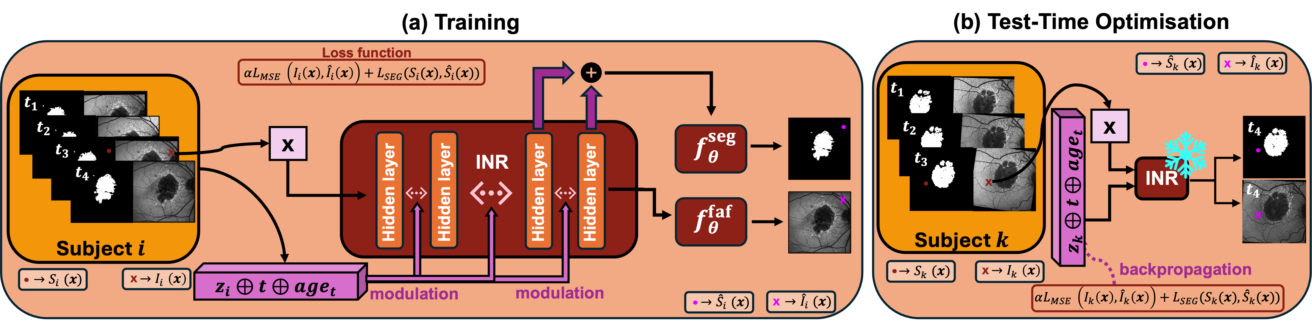
Overview of the GAP-INR architecture

Our proposed model architecture. In the training phase (a), a spatial coordinate $\mathbf{x}\in\mathbb{R}^2$ is fed into the MLP. Each layer of the MLP is conditioned by concatenating the latent vector $z_i$, the time in weeks from the baseline visit, $t$, and the age of the patient at $t$, $\text{age}_t$, via modulation. The shared INR is split into reconstruction head $f_\theta^{\text{faf}}$, which outputs the pixel intensity value $\hat{I}_i(\mathbf{x})$ (purple cross in the output FAF), and the segmentation head $f_\theta^{\text{seg}}$, which takes the outputs from the last two hidden layers and outputs the GA segmentation label $\hat{S}_i(\mathbf{x})$ (purple point in the output segmentation). The predictions are compared to the ground truth $I_i(\mathbf{x})$ (red cross in the input FAF) and $S_i(\mathbf{x})$ (red point in the input segmentation), respectively, using a combination of MSE ($\mathcal{L}_{\text{MSE}}$, for FAF reconstruction) and sum of DICE and Binary Cross Entropy ($\mathcal{L}_\text{SEG}$, for GA segmentation) as loss function. During test-time optimisation (b), a new latent vector $z_k$ for a new eye $k$ is randomly sampled from $\mathcal{N}(0,10^{-2})$ and optimised across both FAF images and GA segmentations using the same loss function, while keeping the INR parameters frozen. By concatenating the new optimised latent vector with the time-conditioning variables, the forward pass generates the new FAF image and GA segmentation at the specified time.

Explore a Patient Trajectory

Predictions of FAF and GA segmentation maps over time for a single eye from the test set. A new latent vector is assigned to this eye and optimised on all visits except the one used for evaluation. Interpolated and extrapolated predictions are obtained by setting the value of the temporal variables (number of weeks from the baseline visits, and age of the patient at that visit) in between two existing visits or beyond the last available visit, respectively.

Hold-out (leave-one-out) Interpolated Extrapolated

Fundus autofluorescence — predicted

GA segmentation — predicted

Hold-out (leave-one-out)

Week	0.0
PSNR	—
SSIM	—
DICE	—
Predicted area	—
GT area	—
Area MAE	—

Show ground truth instead of the prediction

The page is static (no model runs in your browser).

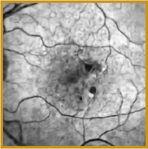
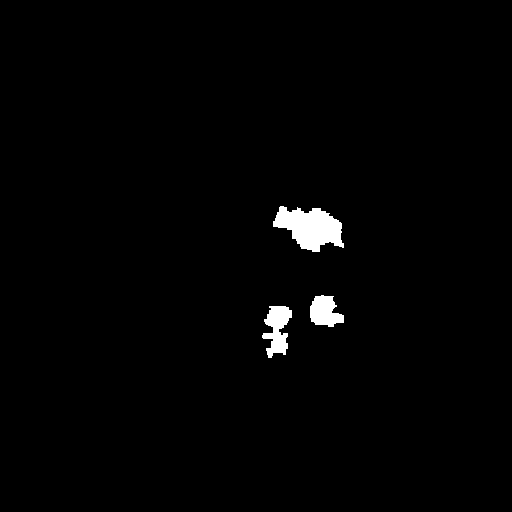
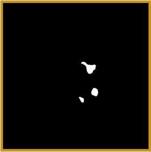
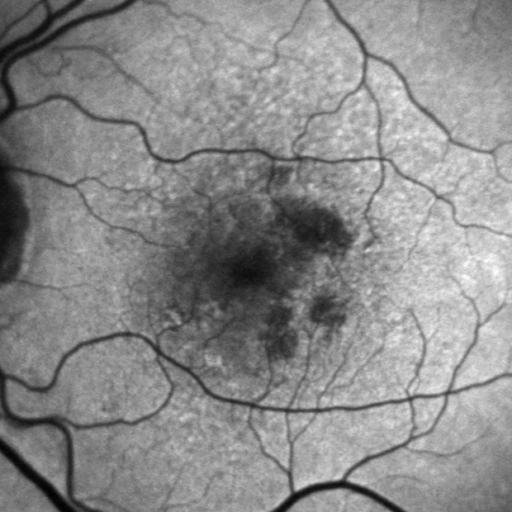
Held-Out Reconstruction — Two Evaluation Scenarios

Our model's predicted FAF image and GA segmentation for an eye from the test set in the two Scenarios explored in the paper: take only a pair of available visits, and use the earlier visit as input to predict the more recent visit (Scenario 1); using the full patient's history to predict the last visit (Scenario 2).

Only the very first visit is given as input to predict the last one.

Prediction Ground truth

FAF: drag anywhere on the image to compare

Prediction Ground truth

Segmentation: drag anywhere on the image to compare

PSNR 16.7 dB · DICE 0.59 · Lesion-area MAE 0.39 mm²

Both scenarios predict Eye A's same last visit, only the input differs. Scenario 1 (V1→V4) is given just the very first visit; Scenario 2 is given the eye's full prior history (V1, V2, V3). That extra context cuts the lesion-area error roughly 19× (0.39 → 0.02 mm²) and raises DICE from 0.59 to 0.82, showing the benefit of taking into account the full patient's history.

Per-Eye Lesion Area Trajectories

Grid of per-eye lesion area scatter plots

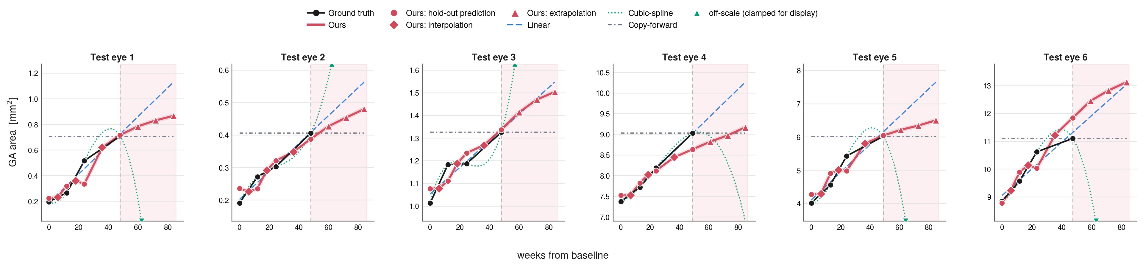
Longitudinal analysis of the individual lesion area trajectories. The six subject-specific predicted trajectories are compared with linear extrapolation, cubic B-spline extrapolation, and copy-forward. Linear and cubic B-spline extrapolation curves are fitted using all ground truth visits.

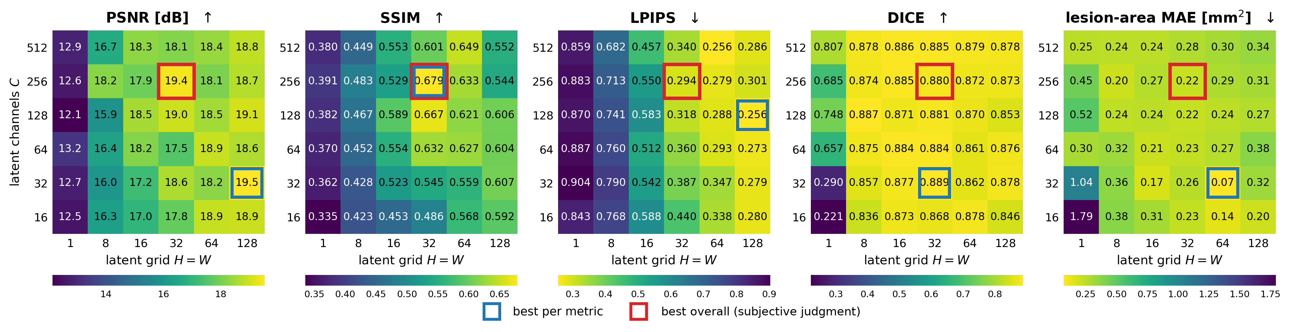
Why monotonicity matters. GA is anatomically irreversible: once tissue atrophies, the lesion does not shrink. Curve fits like linear or cubic B-spline have no mechanism to enforce this and can predict area decreasing between visits; a faithful model's predicted trajectory should stay non-decreasing along each eye's own timeline, not just accurate at the sampled points.

Latent Capacity Ablation

Channel count and spatial grid size of the per-eye latent, swept jointly.

Heatmap of held-out performance across latent channel count and spatial grid size

Latent-grid ablation over number of channels $C$ (rows) and spatial resolution $H\!=\!W$ (columns). Each cell reports a metric at the checkpoint with the best DICE + lesion-area-MAE trade-off (lighter is better). The red box is the best configuration ($C{=}256$, $H{=}W{=}32$) by subjective judgment over all five metrics.

BibTeX

@misc{sarrocco2026modellinggeographicatrophyprogression,
      title={Modelling Geographic Atrophy Progression using Implicit Neural Representations},
      author={Simone Sarrocco and Paul Friedrich and Florentin Bieder and Christina Bornberg and Philippe Valmaggia and Peter Maloca and Philippe Cattin},
      year={2026},
      eprint={2608.10807},
      archivePrefix={arXiv},
      primaryClass={cs.CV},
      url={https://arxiv.org/abs/2608.10807},
}